Explain the methods, show your working and interpret results in context.
Foundation shows shared notes and questions. Higher includes the labelled extensions. Maps and checklist downloads include labelled Higher content; the worksheet generator filters individual goals.
Revise the key ideas
Range, quartiles and percentiles
Range — Subtract the minimum from the maximum. For 4, 7, 8 and 20 the range is 16. It uses only extremes, so one unusual value can change it substantially. Keep the original unit; spread describes variability, not a typical value.
Quartiles — Quartiles divide ordered data into quarters. For a small list state a consistent method, such as medians of lower and upper halves excluding a lone overall median. Different accepted conventions can give different interpolated boundaries; show working, especially when positions lie between observations.
IQR — Interquartile range = Q3 − Q1 and measures the spread of the middle 50%. With Q1=12 and Q3=19, IQR=7. It is less affected by extremes than the range; a smaller IQR indicates a more concentrated middle half, not necessarily a smaller overall range.
Percentiles — The pth percentile is a value at or below which approximately p% of the data lie. Read the p/100 × n cumulative position on a grouped curve. A 90th-percentile time of 45 minutes is a time boundary, not a claim that 90% take exactly 45 minutes.
Inspect unusual values — An outlier is unusually far from the rest in context. Check the source, units and collection circumstances before deciding if it is erroneous. Correct verified errors; retain genuine unusual data or explain a justified separate analysis. Automatic deletion can distort conclusions.
Compare median and IQR — Pair median with IQR for resistant comparisons. A group with median 30 and IQR 4 has a higher typical value and less middle-half variation than one with median 25 and IQR 9. Quote both measures and interpret them using the variable; neither summary alone describes all observations.Median and middle-half spread. Original illustrative diagram; numerical datasets are fictional worked examples.Enlarge diagram
Transforming spread — Adding the same constant to all values shifts quartiles but leaves range and IQR unchanged. Multiplying all values by positive k multiplies spread by k. Celsius to Fahrenheit multiplies spread by 1.8; the extra 32 changes centre only.
Higher — standard deviation and outlier rules
Interpercentile ranges — Subtract the chosen lower percentile from the upper one. P90 − P10 is the interdecile range, covering the middle 80%; P95 − P5 covers the middle 90%. State the chosen endpoints so different ranges are not compared as if identical.
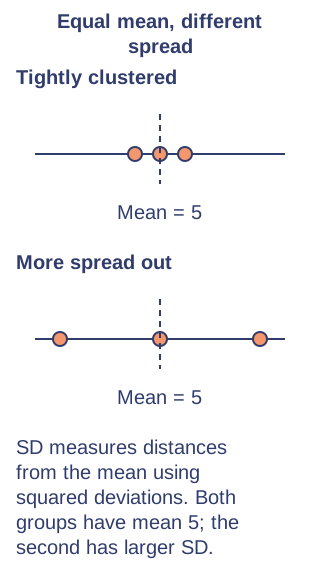
Variance and SD — Population variance is the mean squared distance from the mean; SD is its square root, returning to the original unit. For 2, 4 and 6 the mean is 4, squared deviations total 8, variance 8/3 and SD ≈ 1.633. Use divisor n for the specification's dataset formula, not n−1.
Frequency SD — For value/frequency data use √(Σfx²/Σf − (Σfx/Σf)²). For grouped data substitute class midpoints and recognise the result is an estimate. Select the population SD calculator output; confusing Σfx² with (Σfx)² produces the wrong result.
SD comparisons — Pair mean with SD: a smaller SD means data are more closely clustered around their mean. SD uses every value and is sensitive to outliers. Translation leaves SD unchanged; multiplication by positive k multiplies SD by k, while variance multiplies by k².
IQR fences — A low outlier is below Q1 − 1.5IQR; a high outlier is above Q3 + 1.5IQR. With Q1=10 and Q3=18, fences are −2 and 30. Equality to a fence is not outside it; the rule flags investigation rather than proving a recording error.
Three-SD rule — Values outside μ ± 3σ are flagged by the three-SD criterion. With mean 50 and SD 4 the interval is 38–62. The rule is a diagnostic; distribution shape and context determine its usefulness and do not justify assuming normality without evidence.
Standardised scores — z = (x − μ)/σ says how many SDs a value lies above or below its mean. A score 70 with mean 60 and SD 5 has z=2. Compare like-for-like measurements and remember whether higher or lower is desirable; z is unitless and undefined if SD is zero.
Test yourself
30 questions · Sets of 10 from the selected tier. For fractions, use / when typing; for powers, use superscripts or ^. Follow each question's answer format. These quick checks support revision; practise full written solutions, graph constructions and enquiries too.
Mind map
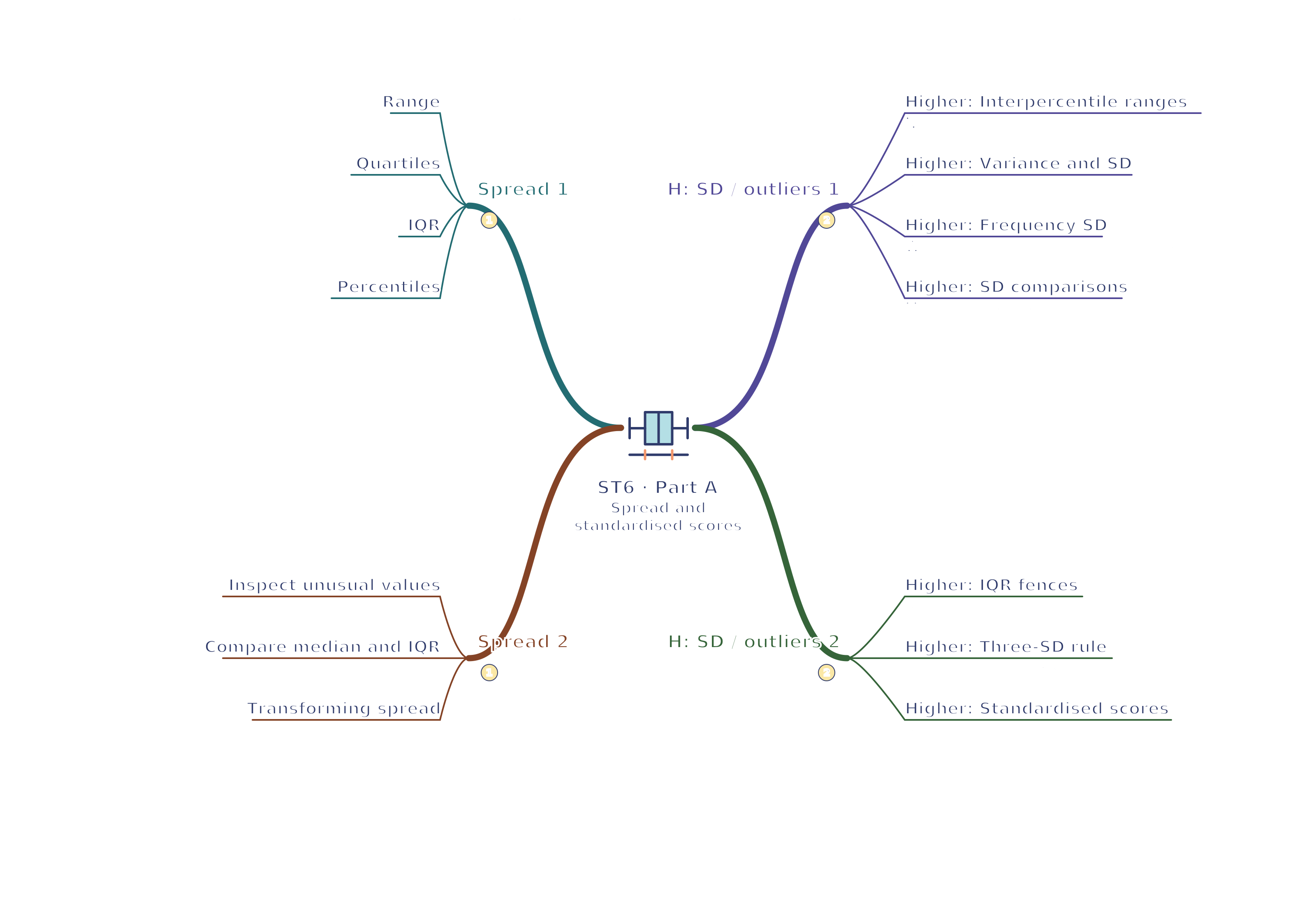
Use the branches to recall the ideas and explain their connections. Check the revision notes for the full detail.
View ST6 · Spread 1 / Spread 2 / H: SD / outliers 1 / H: SD / outliers 2 mind mapOpen the full-size map to zoom. Download the PDF to print on A4 or enlarge to A3.
 Mr Kidman's Classroom